This tutorial is about calculating the R-squared in Python with and without the sklearn package.
For an exemplary calculation we are first defining two arrays. While the y_hat is the predicted y variable out of a linear regression, the y_true are the true y values.
import numpy as np

y_hat = np.array([2,3,5,7,2,3,8,5,3,1])
y_true = np.array([5,4,2,7,4,2,1,6,5,3])
Now we are calculating the R-squared out of those two variables.
The formulas for calculating the R-squared are:
where SST is:
and SSE is:
To understand the SST and SSE consider the following image found on Wikipedia and created by Orzetto (Please see the credits and license below the image):
Attribution: Orzetto / CC BY-SA (https://creativecommons.org/licenses/by-sa/3.0)
On the left-hand side, you see the SST – the total sum of squares which are just the squared differences between the actual y values and the mean y.
On the right-hand side, you see the SSE – the residual sum of squares which is just the summed squared differences between the regression line (m*x+b) and the predicted y values.
You can also just use the sklearn package to calculate the R-squared.
from sklearn.metrics import r2_score

r2_score(y_true,y_hat)
For an application of the R-squared on real data, you are kindly invited to check out the video on my channel
Matplotlib is one of the most popular library for data visualization and that’s for a reason. It has so many features to offer and can be used without any external software except python and the matplotlib library.
In this article, you will learn how to use matplotlib to visualize data that will also enable you to better understand the data, extract information, and make more effective decisions.
Before going further into matplotlib, let’s talk about Data Visualization
What is Data Visualization?
“A picture is worth a thousand words.” We are all familiar with this expression. It especially applies when trying to explain the insights obtained from the analysis of increasingly large datasets. Data visualization plays an essential role in the representation of both small and large-scale data.
Data visualization is the graphical representation of information and data. Graphical representation(in the form of charts, graphs, and maps etc) allows us to better understand the relationship in the data, data visualization tools provide an accessible way to see and understand trends, outliers, and patterns in data
One of the key skills of a data scientist is the ability to tell a compelling story, visualizing data and findings in an approachable and stimulating way.
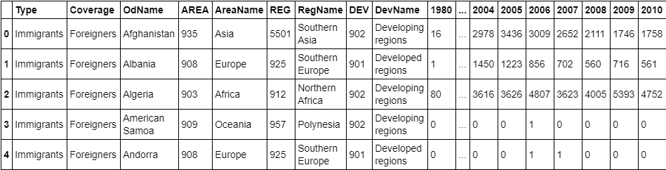
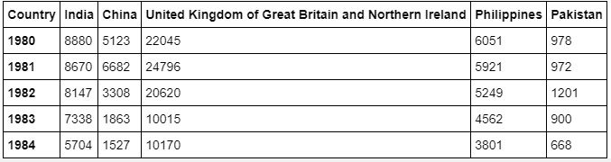
The dataset contains annual data on the flow of international immigrants as recorded by the countries of destination. The data presents both inflows and outflows according to the place of birth, citizenship or place of previous / next residence both for foreigners and nationals. The current version presents data pertaining to 45 countries.The dataset is available here.
Downloading and Preparing Data
import pandas as pd           #For reading the data

#Read the dataset skipping top 20 rows(irrelevant) and second last row
df_canada = pd.read_excel("./data/canada.xlsx",skiprows = range(20),skipfooter=2) df_canada.head() #View top 5 rows
#Check the dimensions of our canada dataset
df_canada.shape # (195, 43)
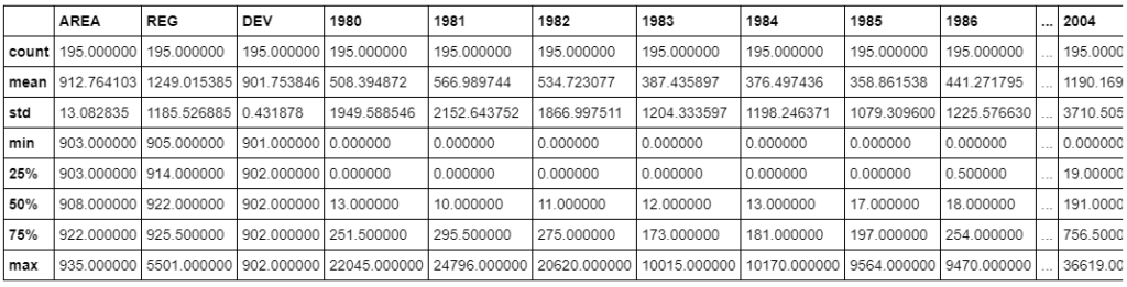
#Let gets insight of our dataset
df_canada.describe()
Cleaning the Dataset
Remove columns that are not informative to us for visualization(eg., type, area, reg)
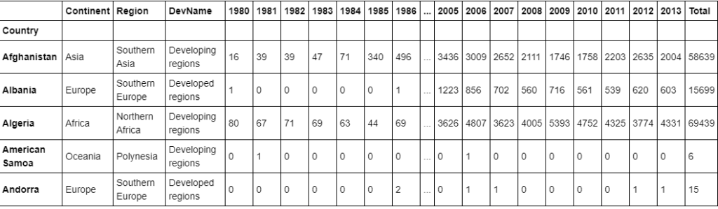
df_canada.rename(columns={"OdName":"Country","AreaName":"Continent","RegName":"Region"},inplace = True)
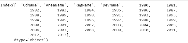
#View columns of our dataset
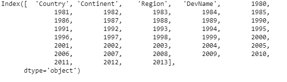
df_canada.columns
Check if column labels are string
For consistency, make sure that all column labels are of type string.
# let's examine the types of the column labels
all(isinstance(column, str) for column in df_canada.columns)
#False

df_canada.columns = list(map(str,df_canada.columns))
# let's examine the types of the column labels
all(isinstance(column, str) for column in df_canada.columns)
#True
Set the country name as index – useful for quickly looking up countries using .loc method.
df_canada.set_index("Country",inplace=True)
Add total column
#Add a column Total in our dataset containing
#total numbers of immigrants
df_canada["Total"] = df_canada.sum(axis=1)

#View top 5 rows
df_canada.head()
Visualizing Data using matplotlib
Now after we have cleaned the dataset, its time to draw some plots. Plotting data using Matplotlib is quite easy. Generally, while plotting they follow the same steps in each and every plot. Matplotlib has a module called pyplot which aids in plotting figure. The Jupyter notebook is used for running the plots. We import matplotlib.pyplot as plt for making it call the package module.
Installing matplotlib
Type !pip install matplotlib in the Jupyter Notebook or if it doesn’t work in cmd type conda install -c conda-forge matplotlib . This should work in most cases.
#import necessary modules
import matplotlib.pyplot as plt

# use the inline backend to generate the plots within the browser
%matplotlib inline
LINE PLOTS
What is Line Plot? When to use Line Plot?
A line chart or line plot is a type of plot which displays information as a series of data points called ‘markers’ connected by straight line segments. It is a basic type of chart common in many fields. Use line plot when you have a continuous data set. These are best suited for trend-based visualizations of data over a period of time.
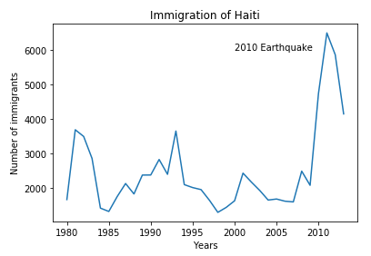
Let’s Start with a Case Study
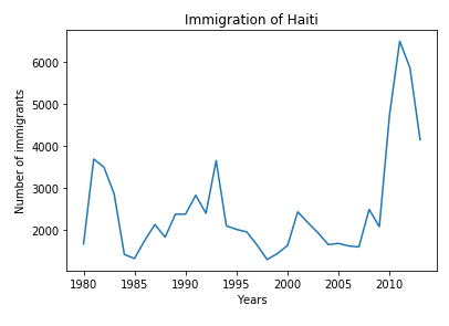
In 2010, Haiti suffered a catastrophic magnitude 7.0 earthquake. The quake caused widespread devastation and loss of life and aout three million people were affected by this natural disaster. As part of Canada’s humanitarian effort, the Government of Canada stepped up its effort in accepting refugees from Haiti. We can quickly visualize this effort using a Line plot:
#First, we will extract the data series for Haiti.
years = list(map(str, range(1980, 2014)))
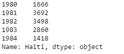
haiti = df_canada.loc["Haiti",years ]
# passing in years 1980 - 2013 to exclude the 'total' column
haiti.head()
pandas automatically populated the x-axis with the index values (years), and the y-axis with the column values (population). However, notice how the years were not displayed because they are of type string. Therefore, let’s change the type of the index values to integer for plotting.
haiti.index = list(map(int,haiti.index))
Also, let’s label the x and y axis using plt.title(), plt.ylabel(), and plt.xlabel() as follows:
haiti.plot(kind = "Line")     #Plotting the line
plt.title("Immigration of Haiti")
plt.xlabel("Years")
plt.ylabel("Number of immigrants")

plt.show() # need this line to show the updates made to the figure
We can clearly notice how number of immigrants from Haiti spiked up from 2010 as Canada stepped up its efforts to accept refugees from Haiti. Let’s annotate this spike in the plot by using the plt.text() method.
haiti.plot(kind = "Line")     #Plotting the line
plt.title("Immigration of Haiti")
plt.xlabel("Years")
plt.ylabel("Number of immigrants")

plt.text(2000,6000,"2010 Earthquake")
plt.show() # need this line to show the updates made to the figure
We can easily add more countries to line plot to make meaningful comparisons immigration from different countries.
Lets Compare the trend of top 5 countries that contributed the most to immigration to Canada.
#Sorting the dataset using sort_values() method
df_canada.sort_values(by = "Total",ascending  = False, inplace = True)

#Extract the data for top 5 countries
years = list(map(str,range(1980,2014)))
df_top = df_canada.head()

#Transpose the dataset
df_top=df_top[years].transpose()
df_top.head()
Now create a line plot and visualize the data
df_top.plot(kind='line')            #Plotting line

plt.title('Immigration Trend of Top 5 Countries')
plt.ylabel('Number of Immigrants')
plt.xlabel('Years')

plt.show()
Final Words
Thank you for the read. I hope that you have enjoyed the article. If you like it, share it with your friends. Also, I have a quick task for you to see how much you have learned. You can think of it as an assignment.
Task. COMPARE THE TREND OF LAST 5 COUNTRIES THAT CONTRIBUTED THE MOST TO IMMIGRATION TO CANADA.
I’ll be happy to hear your feedback. If you have some questions, feel free to ask them. 😉
Hey guys, this is the fourth tutorial of the Python for Beginners Series. If you haven’t checked out our previous tutorials, you should go and check them for a better understanding. In this tutorial, we are going to discuss the statements and escape sequences. This tutorial is focused on statements so you will learn about statements in general and then comments, what are comments, how to write comments in Python, docstrings, escape sequences, and the python blocks.
So, without further ado, let’s start now.
Statements
Any instruction that you give to python to execute is a statement. You say
print("Hello World")
This is a print statement because you are printing some data, which in this case is a string. Anything you write is a statement. You assign a value to a variable, that’s a declaration/assignment statement. Now some of you might have heard about if, else, for, while, etc… These all are statements.
Now statements can be of single-line or multi-line. Till now, you may have only used single line statements like print(“Hello World”) but there are multi-line statements as well.
Multi-Line Statements
You can extend a single statement to multiple lines. Try making a multi-line statement like this one.
a = "Coding
Ground"
print(a)
It will throw an error like
    a = "Coding
              ^
SyntaxError: EOL while scanning string literal
To extend the statement to multiple lines, all you have to do is put a backslash ( \ ) at the end of the statement. For example,
a = "Coding\
 Ground"
print(a)
And the output will be
Coding Ground
You can also put your statement under brackets for some data types and you won’t need to use backslash but it is not true for strings. For example
a = ['item1',
'item2']
print(a)
The output will be
['item1', 'item2']
It will work with tuples as well.
Now you might be wondering why should we even use it when we can just write it in one line. Well, it is done to make your code cleaner and increase its readability.
Comments
You must have noticed that in some code there is a text written beside it which describes what the code is for. That text is called a comment. There are two types of comments, single-line comments which are normal comments and multi-line comments which are also known as docstrings
Single Line Comments
These are written in a single line for example,
a = "Coding Ground" #Assigns value to variable a
Single Line comments start with a hashtag. They are written to describe what the code is about, it’s working what the variable stores and so on. Comments are only for user understanding and are never executed with the code.
You can write as many comments as you would like and it’s a good practice to write comments so that others can understand your code without much hassle. Not only for other people, but it will also help you in reading your code after a long time.
Docstrings or Multi-Line Comments
There are times when you have to add a full documentation about a function or a class you create or sometimes, it’s just that you have to write multi-line comments, for that we use docstring.
Docstring is any text written under triple quotes like ”’ or “””. For example,
"""This is a
docstring"""
'''This
is
also a
docstring'''
If you want to add a documentation of a function you can do this like
Docstring for functions, classes, or modules is written right after their declaration before any other statement.
Now if you want to access the documentation of a function/class/module, all you have to do is call the attribute __doc__.
You can, in this case, do this by printing function.__doc__. For example,
print(codinground.__doc__)
It will print out whatever is written in the docstring of that function or module or class. It will be really helpful whether you are experienced or beginner in python.
The output in this case will be
prints Coding Ground
So, docstrings will help you write documentations in an efficient and a standard way for everyone to follow.
Now, this isn’t a norm but a personal preference that you should write docstrings when you are writing a function or a class or module and single-line comments when you are writing loops or variables.
You might be confused about functions, classes, or modules but don’t worry, we’ll be covering them in our future tutorials in this series. But if you are confused about variables, I recommend checking out our tutorial on Datatypes and Variables in Python
Coming over to our next topic which is Escape Sequences.
Escape Sequences
There are some characters in python which have a different meaning. These are called escape sequences and are written after the escape character backslash( \ ).
For example, if I told you to print out a string whose output is “Coding Ground”. How would you do it? simply using print(“”Coding Ground””) will throw a Syntax Error.
There are many such cases where we want our text to be under quotes or in a new line without actually writing it in another line etc., in these cases, we use escape sequences.
To print a text under quotes just put a backslash before the quotes.
print("\"Coding Ground\"")
The output of this will be “Coding Ground”. This is because the double quotes are written after the escape character backslash. If you try to put backslash without any other character, it will leave whitespace. The backslash defines that the character after after the escape character has a different meaning than the normal one.
TIP If it’s just printing the text under double or single quotes you can just do it like this print(‘”Coding Ground”‘). What I have done is, I started the string with a single quote and wrote the word under double quote so python interpreter knows that ok, the main string is whatever text is under single quotes. So, it treats double quotes as an ordinary string character. But this is not recommended
You can also use \n to make it the next line. I know this is not clear so let’s consider this example, You are making a menu for your program and you want to list multiple items in it. Then you can do this by using the \n like
print("1. Item One\n2. Item Two\n3. Item Three")
The output of this will be
1. Item One
2. Item Two
3. Item Three
You can see that it is much more efficient than writing it in multiple lines.
Similarly, there are many such escape sequences, you can find a list of them below.
Escape Sequence
Meaning
\newline
Backslash and newline ignored
\\
Backslash (\)
\'
Single quote (')
\"
Double quote (")
\a
ASCII Bell (BEL)
\b
ASCII Backspace (BS)
\f
ASCII Formfeed (FF)
\n
ASCII Linefeed (LF)
\r
ASCII Carriage Return (CR)
\t
ASCII Horizontal Tab (TAB)
\v
ASCII Vertical Tab (VT)
\ooo
Character with octal value ooo
\xhh
Character with hex value hh
List of Python supported Escape Sequences
These are all the escape sequences available in Python. Play with them and you will have a better understanding.
Python Blocks
In our previous example on docstring, we made a function and then wrote a docstring. If you have noticed carefully then you must be wondering why we put a colon after the function definition and then we leave two spaces in the statement we wrote under that function?
This is because unlike other languages, which use curly braces {} to define a block, python uses colon and indentation which is usually two or four spaces.
According to Python’s Official Documentation,
A block is a piece of Python program text that is executed as a unit. The following are blocks: a module, a function body, and a class definition. Each command typed interactively is a block.
All conditional statements, functions, classes and modules use a python block.
Let us look at a if statement to make it more clear.
 a = 10
 if a == 10:
    print("This code executes under if block")
print("This executes anyway")
Since the condition is true, which is a is equal to 10, if block will run and the output will be
This code executes under if block
This executes anyway
If we tweak the value of variable a, suppose 1, then the if condition will become false and if block will not run and the output will simply be
This executes anyway
So basically, a block is a piece of code that executes as a unit whenever called.
Hopefully it should have given you some basic insight on loops as well.
We will discuss python blocks in detail when we cover control flow statements.
This is it for this tutorial, hope you like it. Tell me what you think of this tutorial in the comments section below. Also, if you have any doubts, comment down below and I’ll help you.
Hey guys, this is the third tutorial of the Python for Beginners Series. If you haven’t checked out our previous tutorials, first go and read them (especially Tokens in Python) because we have discussed keywords and identifiers in those tutorials that you should know before learning about variables.
What are variables?
Variable is a name that points to a location where your data is stored. In simple language, the variable holds your data. You can assign a value to a variable using = sign with the variable on left and value on the right. Consider this example,
age = 10
In this example, age is a variable that points to the memory location where the data i.e., 10 is stored. Now whenever you want to use 10, you can also use variable age.
For example, if you do this
print(age)
The output will be 10
Also, it is important to know that the data inside the variable can be changed whenever you need. For example, you could store a value 20 in the same variable.
age = 20
Now the variable age holds value 20. The old value 10 is now replaced by the new value 20.
You can store all sorts of data in a variable like
name = "Coding Ground"
the variable name holds the string value Coding Ground.
It is important to remember that variables do not store values they are the pointers. They give reference to the memory location where the data is stored.
Before we dive any deeper, let us discuss the different type of data supported in python.
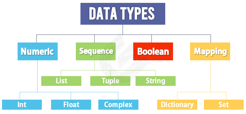
DataTypes
A datatype is simply the attribute of data that tells the interpreter what type of data it is going to process.
There are multiple data types supported in Python. Also, you can check the type of data using the type() function.
Python Data Types
Numeric Data
The numeric data type includes integers, floating-point numbers, and complex numbers. They are used as int, float,and complex. Consider the examples below,
Integers
These are the whole numbers which also include negative numbers. For example, 0,1,2,3,150, -200 etc are all integers. They don’t have a fraction part.
a = 10
print(type(a))
It will return
<class 'int'>
Floating Point Numbers
Floating Point numbers have a decimal part in them.
b = 10.2
print(type(b))
The output will be
<class 'float'>
Complex Numbers
These numbers are in the form of a + bj. They are as <real part> + <imaginary part>j
c = -1 + 5j
print(type(c))
The Output will be
<class 'complex'>
Now you see class because the data is an object or instance of a class. For example, 10 is an instance of int class.
If you don’t understand it then don’t panic, We will be discussing classes and objects in future lectures.
Sequence
Sequences include lists, tuples and strings. Basically every data type in which slicing can be done falls under this category.
Lists
Python lists contains elements within square brackets [ ].
a = ["Coding Ground",1,1.2,True]
print(type(a))
The Output would be
<class 'list'>
In the above example, the variable a holds a list of 4 elements, each of different data type.
Now each element of list has an index value and it starts from 0.
For example, the index value of the element “Coding Ground” in the above code will be 0.
We will discuss indexing and slicing in future tutorials.
Tuples
Tuples contain elements in round brackets or parenthesis ( ).
An example of a tuple would be
a = ("Coding Ground",1,1.2,True)
print(type(a))
The output would be
<class 'tuple'>
Now you might be wondering, what is the difference between list and tuple?
The answer is that Lists are mutable while tuples are not. That means you can change the elements of a list without replacing the whole variable value but you can not do that with tuple. You can not perform operations on them.
String
Anything within single or double quotes in Python is a string.
a = "Coding Ground"
print(type(a))
The output would be
<class 'str'>
Boolean
Boolean on values can only be either True or False.
a = True
print(type(a))
The Output will be
<class 'bool'>
Remember that True is a keyword and T is capital.
Mapping
There are 2 types of Data Types that fall under this category. These are Dictionary and Sets.
Dictionary
Dictionary is an unordered collection of key-value pairs. It uses curly braces. If you’ve ever worked with JSON data then you must be familiar with Dictionary.
a = {'name' : "Coding Ground"}
print(type(a))
The Output will be
<class 'dict'>
Dictionaries provide a little more readability as compared to lists and tuples. This is because of the key-value pair. And this is the reason they are used when we have to work with a large amount of data.
Sets
Like dictionaries, Sets are also unordered collections with curly braces. But the difference is that they contain only unique values.
a = {1,2,3,4,5,1,2,3}
print(a)
print(type(a))
The output would be
{1, 2, 3, 4, 5}
<class 'set'>
Here, you can clearly see that we got only unique values as the output.
We cannot filter data from sets as sets are unordered pair. We can however use the classic set functions like union, intersection etc on two set values.
Now that we have discussed the data types, lets continue where we left the variables.
Type Casting or Type Conversion
Now that you have learnt about the different data types and how to assign a value to a variable. It is time to learn how you can convert the data type of some data stored in a variable.
Consider this example,
a = 10
print(a)
print(type(a))
a = float(a)
print(a)
print(type(a))
The output will be
10
<class 'int'>
10.0
<class 'float'>
As you can see we have just converted an integer value to a float one. But remember that you can not do this with all data. You can only do this with data having similar data type.
Now this is all common sense, I don’t need to explain this. If you are thinking how about converting complex to int or float, it won’t work because complex got j in it which isn’t used in any int value or float value.
But you can convert string into a list.
a = "Coding Ground"
a = list(a)
print(a)
print(type(a))
Hey Guys, this article will give you a quick introduction of pandas as to what is Pandas, why you should use Pandas, what can you do with Pandas, and the supported Pandas data types. It can help you make sure if Pandas is what you are looking for or you should learn pandas or not.
If you’re looking for data science then you must have heard of this library at least once. Pandas is the most famous/downloaded library for data science. Why? Because it is super fast and makes working with datasets so much easier. We’re gonna talk about everything from series to DataFrames, from creating a new DataFrame to reading an old dataset everything.
Prerequisites
You should have a basic understanding of Python especially dictionaries, lists, and tuples. Some basic knowledge of NumPy will also be helpful as arrays are often used in Pandas Series and DataFrames along with the dictionaries. If you want to learn NumPy then check out our amazing tutorial on NumPy Arrays which covers everything that you need to know about NumPy.
What is Pandas?
Pandas is a high-performance open-source library for data analysis in Python developed by Wes McKinney in 2008. Over the years, it has become the de-facto standard library for data analysis using Python.
Why Pandas?
The benefits of pandas over using the languages such as C/C++ or Java for data analysis are manifold:
Data representation : It can easily represent data in a form naturally suited for data analysis via its DataFrame and Series data structures in a concise manner. Doing the equivalent in C/C++ or Java would require many lines of custom code, as these languages were not built for data analysis but rather networking and kernel development.
Data sub-setting and filtering : It provides for easy sub-setting and filtering of data, procedures that are a staple of doing data analysis.
Features of Pandas
It can process a variety of data sets in different formats: time series, tabular heterogeneous arrays, and matrix data.
It facilitates loading and importing data from varied sources such as CSV and DB/SQL.
It can handle a myriad of operations on data sets: sub-setting, slicing, filtering, merging, groupBy, re-ordering, and re-shaping.
It can deal with missing data according to rules defined by the user and developer.
It can be used for parsing and managing (conversion) of data as well as modeling and statistical analysis.
It integrates well with other Python libraries such as stats models, SciPy, and Scikit-learn.
It delivers fast performance and can be speeded up even more by making use of Cython (C extensions to Python).
Setting Up
Now, I’m not a big fan of Jupyter Notebook but it makes the data science easier to understand because you know exactly which block is executing which code.
Since most people find it difficult to use Jupyter Notebook standalone without Anaconda, We’ll stick to our old favorite – Default IDLE
Installing Pandas and JupyterLab
Now for those who do want to use Jupyter Notebook, if you have anaconda installed, it’s fine to skip the whole setting up section because Pandas comes pre-installed with Anaconda. If you don’t have Anaconda, continue reading
This is it, it will install Jupyter Notebook in your system. Also, you may also be aware that there’s a jupyter library too. We aren’t going to install that because it is no longer updated and this just gets the job done fairly well.
Check out this video. It might help you set up Jupyter Lab
Now, I won’t be explaining how to use Jupyter Notebook here in this tutorial because this is out of the scope of this tutorial. So, we’ll just get to the point. Open your terminal, cd to the path where you want to access files using Jupyter, and open Jupyter Notebook there. I will make a video on that in future tutorials but this article is about Pandas so we’re gonna skip that.
Now all you have to do is install Pandas. It is fairly easy to do so. Just open pip and type
pip install pandas
This will install pandas in your computer.
Syntax
The general convention is that you import pandas with an alias name pd. It is not necessary that you import it with this name but it is the recommended way to do it and you’ll find it this way in most of the places. So, it will improve readability of your code.
import pandas as pd
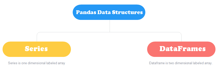
Pandas Data Structures
Pandas supports two main type of Data Structures. Series and DataFrames!
Series
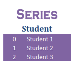
Pandas Series is the one-dimensional labeled array just like the NumPy Arrays. The difference between these two is that Series is mutable and supports heterogeneous data. So Series is used when you have to create an array with multiple data types. Imagine a table, the columns in that table are Series and the table is a DataFrame.
Take a look at the image below. It will help you visualize better.
Series Example
Creating Series
Syntax for creating Pandas Series is:
import pandas as pd
s = pd.Series(data=None, index=None, dtype=None, name=None, copy=False, fastpath=False)
NOTE: ‘S’ of the pd.Series is capital. People tend to forget that.
This syntax may seem a little overwhelming but you do not need to focus on all the parameters. Most of the time you will only be using the data and index parameters but we will be discussing all the parameters here. But let’s first create example Series here.
import pandas as pd
s = pd.Series(["Coding Ground",1,5.8,True])
print(s)
Output will be:
0    Coding Ground
1                1
2              5.8
3             True
dtype: object
Now that we have a Series of consisting data of multiple datatypes, we can proceed further.
data: Sequence, most preferably list but can also be dictionary, tuple, or an array. It contains data stored in Series.
index: This is optional. By default, it takes values from 0 to n but you can define your own index values. Now there are two ways to define index,
s = pd.Series(["Coding Ground",1,5.8,True],index=["String","Integer","Float","Boolean"])
And it will work same as defining index in parameters. Output will be
1    Coding Ground
2                1
3              5.8
4             True
dtype: object
dtype: It is the datatype of the Series. If not defined, it will take values from the series itself. If it’s the same for all element, it will show a specific data type such as int else it will show Object.
name: It is the name given to your pandas series
s = pd.Series(["Coding Ground",1,5.8,True],index=["String","Integer","Float","Boolean"],name="Pandas Series")
It will add a name “Pandas Series” to your Series. The output will be
You can also do the same using s.name = “Pandas Series”
copy: It creates a copy of the same data in variable(s). By default it is set to False i.e., if you change the data in one variable, it’ll change in all variables wherever the data is stored. Change it to True and all the locations where the data is store will be independent of each other. For example,
s = pd.Series(["Coding Ground",1,5.8,True],index=["String","Integer","Float","Boolean"],name="Pandas Series")
ss = s
ss[1] = 2
print(ss)
print(s)
You can clearly see that even though you changed the value of the second element in ss, it automatically got changed in s. This is because copy by default is False. Set it to True
ss = s.copy()
ss[1] = 3
print(ss)
print(s)
This will create a new copy in ss and they will not share same data location point anymore. So, changing one will not change another.
fastpath: Fastpath is an internal parameter. It cannot be modified. It is not described in pandas documentation so you may have to take a look here.
DataFrames
DataFrame is the most commonly used data structure in pandas. DataFrame is a two-dimensional labeled array i.e., Its column types can be heterogeneous i.e. of varying types. It is similar to structured arrays in NumPy with mutability added. It has the following properties:
Similar to a NumPy ndarray but not a subclass of np.ndarray.
Columns can be of heterogeneous types e.g char, float, int, bool, and so on.
A DataFrame column is a Series structure.
It can be thought of as a dictionary of Series structures where both the columns and the rows are indexed, denoted as ‘index’ in the case of rows and ‘columns’ in the case of columns.
It is size mutable that means columns can be inserted and deleted
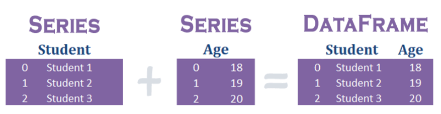
Suppose now you want to change the columns from “student” to “name of student” and from “Age” to “Age of Student”. You could do it easily as:
df.columns = ["Name of Student","Age of Student"]
And the output will be
           Name of Student  Age of Student
row1        Student1              18
row2        Student2              19
row3        Student3              20
So, this is it, we have covered all the parameters of DataFrames along with an example.
dtype: The datatype of Data in the DataFrame
copy: Same usage as Series, allows different location of same data.
We aren’t going to discuss the copy parameter here because that would require a lot of examples and new functions which are out of scope of this tutorial. We will be discussing these things in details in the future lessons.
Conclusion
Congratulations on completing this tutorial. It was your first step in deciding whether you should learn Pandas or not and since you’re reading this, you made the right choice.
Personally, I recommend learning Pandas because why not? It is the most powerful library and if data science is what you’re aiming for then you’ll see this library a lot.
You should set up Jupyter Notebook or preferably Anaconda. Use IDLE only if you can’t have Jupyter Notebook or Anaconda. IDLE will be a little bit slower when processing data compared to Anaconda but that’s fine. I mean you don’t necessarily need it but it will help you understand better. Also one more thing, remember that S of pd.Series and D of pd.DataFrame is in caps. People make that mistake a lot and their program fails.
So, now I want to ask you, can you make a DataFrame using Series? If yes, how? Comment down the answer below!
So, guys, this is it for this tutorial, we’ll be looking at more advanced topics in the future.
Hey guys, this is the second tutorial of the Python for Beginners Series. If you haven’t read the first one i.e, Getting Started with Python yet then I suggest checking that out first. Also, this is going to be mostly theoretical with almost no coding involved but is very important. Do not skip this if you don’t know about tokens in Python.
The Python Character Set
It is the set of valid characters that python understands. Python uses the Unicode character set. It includes numbers from numbers like Digits: 0-9, Letters: a-z, A-Z Operators: +,-,/,*,//,** Punctuators like : (colon), (), {}, [] Whitespaces like space, tabs, etc
What are tokens?
Tokens are building blocks of a language. They are the smallest individual unit of a program. There are five types of tokens in Python and we are going to discuss them one by one.
Types of Tokens
So the five types of tokens supported in Python are Keywords, Identifiers, Literals, Punctuators, and Operators. Coming over to the first one we have
Keywords
Keywords are the pre-defined set of words in a language that perform their specific function. You cannot assign a new value or task to them other than the pre-defined one.
You cannot use them as a variable, class, function, object or any other identifier.
For example: if, elif, while, True, False, None, break etc
These have their special task that you cannot change. For example break will only end the loop you cannot make it start the loop. (We’ll be covering loops in future lectures).
Identifiers
Now identifiers are the names that you can assign a value to. An identifier can be anything for example,
a = 10
Here, a is a valid identifier name. Any name you give your variable, function, or class is an identifier of that particular thing. Now there are certain rules that you have to follow to define a valid identifier name.
Rules for valid identifier name
A valid identifier name can have letters, digits, and underscore sign.
It can start with an alphabet or underscore but can never start with a digit.
It can never be a keyword name.
An identifier name can be of variable length.
The only special symbol that can be used in identifier name is underscore( _ ).
One more thing that you should remember that python is case sensitive i.e.,
a = 10
A = 5
These two hold two different values. a holds the value 10 and A holds the value 5.
Examples of valid identifier names include: a, _a, a12, etc Examples of invalid identifier names include: 1a, $a, elif, print. If you don’t understand why they are valid/invalid, read the rules again.
Literals
Literals are the fixed or constant values. They can either be string, numeric or boolean.
For example, anything within single or double quotes is classified as a string and is literal because it is a fixed value i.e, “Coding Ground” is literal because it is a string.
Another example is, 10. It is a simple number but is a fixed value. It is constant and it will remain constant. You can perform operations like addition or subtraction but the value of these two characters 1 and 0 put together in a correct order gives them a value equal to ten and that cannot be changed.
Boolean only consist of 2 values, True and False. Remember that “T” of True is capital. Python is case sensitive and if you write True with small “t” like true it will hold a different meaning. It will act as another variable.
It might seem a bit confusing for now but you’ll definitely understand it in our future lectures on boolean and other data types.
Punctuators or Separators
Punctuators, also known as separators give a structure to code. They are [mostly] used to define blocks in a program. We will be covering code blocks in control flow statements when we discuss how to apply conditions in Python. Some examples of punctuators include single quotes – ‘ ‘ , double quote – ” ” , parenthesis – ( ), brackets – [ ], Braces – { }, colon – ( : ) , comma ( , ), etc. Punctuators and operators go hand in hand are used everywhere. For example,
name = "coding ground"
Here, an assignment operator ( = ) and punctuator, (” “) is used.
And now for the last type of token is Operators
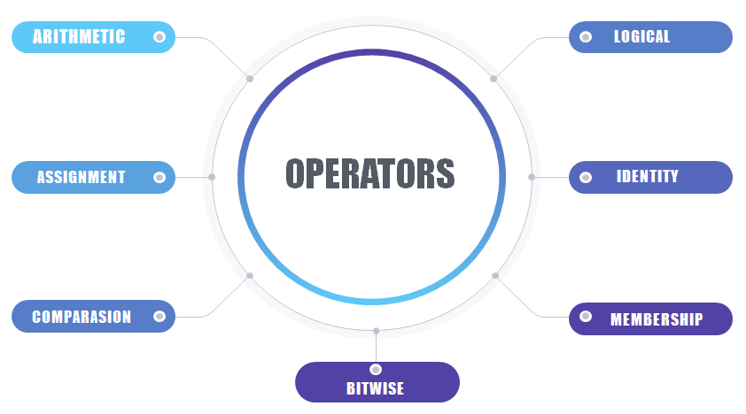
Operators
Operators are the symbols which are used to perform operations between operands.
Unary Operators: Operators having single operand. Eg. +8, -7, etc Binary Operators: Operators working on 2 operands. Eg. 2+2, 4-3, 8*9, etc Similarly, there are Ternary Operators that work on 3 operands and so on. These are just basics and not so important to know but the operators listed below are very important
Arithmetic operators ( +, -, /, * etc)
Assignment operators ( = )
Comparison operators ( >, <, >=, <=, ==, !=)
Logical operators ( and, or, not)
Identity operators ( is, is not)
Membership operators ( in, not in)
Bitwise operators ( &, |, ^ etc)
There’s so much about operators that it cannot be written here as it will be out of the scope of this topic. A new detailed article on tokens will be there very soon.
Hey Guys, if you ever wanted to learn python but you don’t have any past experience then continue reading. This is the first tutorial of Python for Beginners series. In this tutorial we will cover the introduction of python following with its uses and applications. You will install and set up python on your computer and write your first program in Python.
Introduction to Python
Python is an interpreted*, high-level, object-oriented, and open-source language developed by Guido van Rossum and first released in 1991. According to a survey conducted by Stackoverflow, Python is the most sought after programming language by developers.
Compiler – It converts the source code into a machine-dependent code completely all at once. Interpreter – Python runs and checks the code line by line. So if an error is detected at suppose line 2, then it won’t run all the way to the end of the script. Unlike Java, which compiles the whole code at once.
Why Python?
Python is an interpreted language, not a compiled language. Due to this, python is easy to debug.
Python is a cross-platform language, it can run on a variety of platforms.
Python is open-source and free.
Python is best for Artificial Intelligence and Machine Learning.
Setting Up
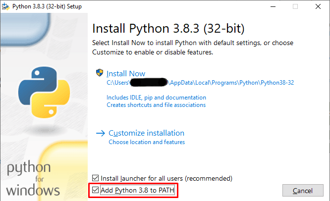
Installing Python is extremely easy, it’s the same as you install any other software. Just go over to the official Python Website and download the latest version or click here.
Remember to check “Add Python 3.X to PATH“. It adds PIP to environment path variables.
PIP is a Python Package installer that helps in installing libraries and modules. You will need it one day or another, so it’s better to install it now.
Selecting the Python IDE(Integrated Development Environment)
Different people suggest different IDE, it all comes down to the personal preferences.
In this series we will be using the default python idle because a large number of people use that and it is generally advised to start with that.
What I recommend is IDLE or Sublime Text. These are more than enough or you can try VS Code. Though there are many other good IDE’s but I believe an IDE should be lightweight and fast because oftentimes you have to use a web browser to search for the problems. So these 3 are the best in terms of speed and efficiency.
Out of these I recommend Sublime Text because it has a large number of color schemes which look fantastic while coding and some people prefer a darker theme which is really great in Sublime.
Working with IDLE
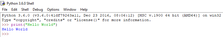
Writing Your First Program
After installation open up Python Shell and write this code.
print("Hello World")
print() function tells Python to print/echo whatever data is in the parenthesis.
In python, string values are written under double quotes. We will be learning more about that in the future lessons.
Congratulations, you wrote your first program in python!
As an assignment, Try printing your name in python.
Working with Files
Most beginners make this mistake of continue writing their whole program in Python Shell. You shouldn’t do it unless you want to perform a quick task.
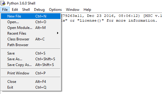
Now in your Python Shell click on File and select New File
Now type the same code in the file and save it. The default extension of python files is .py.
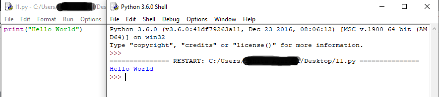
After Saving the file press F5 or click on Run and select Run Module.
It should look something like this. If this is what you got then congrats, you successfully learned how to use python files.
Whether you are building a game or even a simple app with user interaction you need to store the data. There are many methods in Python which are used to store data but by far the most popular one is using MySQL Database. The reason is that it is really easy to use and you can use the SQL file anywhere with any language you like and it is more secure than the others.
What exactly is MySQL?
Databases store the data in tabular form. MySQL is one such Relational Database Management System(RDBMS) for SQL.
Prerequisites
One should have a basic knowledge of both Python and SQL for better understanding.
What’s in this tutorial?
In this tutorial, you will learn how to use MySQL Database with Python. We will make a simple school database consisting of data of students. We’ll store student’s information and retrieve it using Python. So by the end of this tutorial, you will be able to make a full python application that uses MySQL database to store and retrieve data using Python.
Setting Up
MySQL doesn’t come pre-installed with the default windows installation so we’ll need to set it up ourselves. As usual, we’ll be using the default IDLE for python for the sake of simplicity. You can use any IDE.
About MySQL server, you might find it a bit confusing to install and use it if you are a first timer.
So if you are an absolute beginner I’d recommend downloading the command line interface of SQL. Even though it is an older version, it can help you to understand better. You can download it from here.
After installing MySQL now it’s time to install the MySQL driver for Python.
For that we’ll be using python mysql connector.
To install mysql connector just open pip and type
pip install mysql-connector
With this you have everything installed correctly. Now let’s get started with the main thing.
Working With MySQL
Connecting Python with MySQL
Now that we have everything installed, we have to make a connection between your Python file and the MySQL database.
First import the module in your python file as
import mysql.connector
This will import the MySQL Driver in python file. Next up connect your file with server.
Where username and password are defined by you. Generally both of them are root.
Now that you’ve established the connection with the server, all you have to do is execute the database commands.
Creating Database
Let us create a database named school. Since my username and password is root, I’ll be using that.
import mysql.connector

#Establishing Connection with MySQL Server
conn = mysql.connector.connect(
    host = "localhost",
    user = "root",
    password = "root"
)
cursor = conn.cursor()
cursor.execute("CREATE DATABASE School")
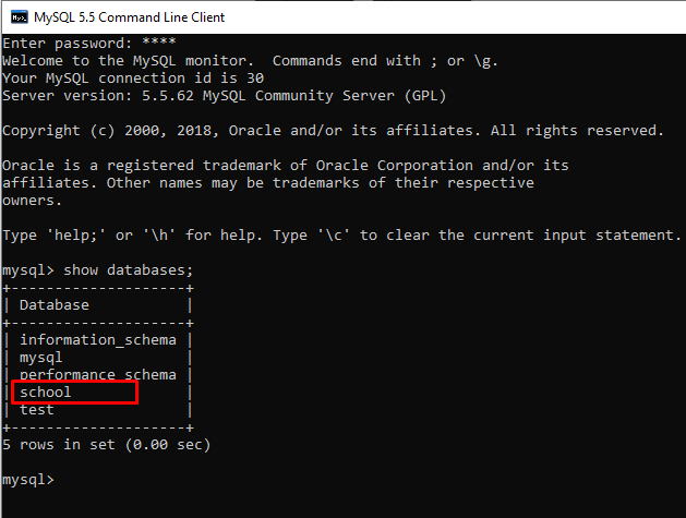
Now open the MySQL Interface, and type show databases; and you will find the school database listed.
Creating Tables
Now that we have database set up, we have to create a table and configure it.
Creating a table is almost similar to the way you create a database. We will make a table named student and store his id, name, email id and username.
cursor.execute("USE SCHOOL")
cursor.execute("CREATE TABLE Student(id int primary key auto_increment,name varchar(20) not null,email varchar(30) unique)")
This will create a sample table Student in the School database.
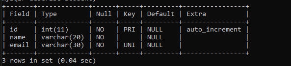
Structure of Student Table
Here we have,
ID – which is kind of a serial number of the registered student. I’ve made it primary key because two students cannot have same serial numbers.
Name – It is the name of the student. Obviously it is a varchar and cannot be null.
Email – It is the email id of the student, it is unique because two students cannot have same email id and they cannot leave it empty.
Now if we ever want to pull specific user data then we can pull it using both id and email since they are unique and will fetch only one result.
Now that we have a table all we need is to make functions for registering and pulling user data.
Storing Data in Tables
First Up, we’ll make a register function
def register():
    name = input("Please Enter Your Name: ")
    query = "SELECT * from Student where email="

    #Checks if the email is already registered
    while True:
    	#Checks if @ is present in email
    	while True:
    		email = input("Enter your email: ")
    		if '@' not in email:
    			print("Invalid Email")
    		else:
    			break
    	tmp_query=query+'"'+email+'"'
    	cursor.execute(tmp_query)
    	result = cursor.fetchall()
    	if len(result) > 0:
    		print("email already registered. Please try again.")
    	else:
    		break
    cmd = "insert into Student(name,email) values (%s,%s)"
    data = (name,email)
    try:
        cursor.execute(cmd,data)
        conn.commit()
        print("Registration Successful")
    except:
        conn.rollback()
        print("Unable to register")
So the code is pretty much self explanatory if you are familiar with python but don’t worry if you are not. We will go through the code
So first we take the student’s name as an input in the name variable then we make a query and store it in the query variable. This is totally optional but it makes string formatting easy to understand.
Now what we did is we applied 2 conditions in the email input. First we check if @ is present in the email because you cannot create an email without @ sign and then we check if the email is already regitered or not.
To retrieve rows from the database we basically have 3 functions.
fetchone() – It fetches the first record that comes up in the query.
fetchmany(number_of_records) – It fetches the specified number of records
fetchall() – It fetches all the records available.
fetchall() and fetchmany() returns a list of tuple whereas fetchone() returns a single tuple. So remember which one you use as it might create error in indexing.
Now after retrieving the records, I stored them into a new variable result and then i checked if the number of records is greater than 0 means there is already one record with that email.
If email is already registered, I prompt user to enter email again as it is already registered using the while loop and breaks if there is no record with that email.
Now there are a lot of ways to check the existence of a particular record but this one just seems to work with me.
In the end, if everything works out fine, I insert the data into the database and commit the data. If by any chance an error occurs, we rollback to previous data.
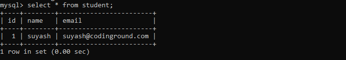
So, I registered with my name and email as suyash@codinground.com
sample table
Quick Tip: While experimenting with the data you might mess up the auto-increment. To reset the auto-increment value run this query: ALTER TABLE Student AUTO_INCREMENT = Value;
You can also run the alter table commands with python this way but you won’t need them very often. So we are not going to use each and every command here instead let us try to retrieve the user data.
Fetching Data From Tables
It will be similar to storing data since we are going to apply same conditions on email check.
def retrieve_info():
	query = "SELECT * from Student where email="
	while True:
		email = input("Enter your email: ")
		tmp_query=query+'"'+email+'"'
		cursor.execute(tmp_query)
		result = cursor.fetchone()
		if len(result) > 0:
			userid = result[0]
			name = result[1]
			print("User ID:",userid)
			print("Name:",name)
			print("Email:",email)
			break
		else:
			print("Email does not exist")
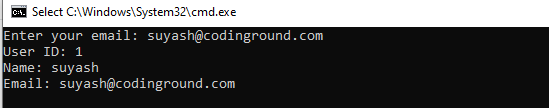
What we did here is we fetched the whole record belonging to that email. Since there were 3 columns in that record(id, name, and email), therefore I stored them into different variables and displayed. It would look like this.
Closing Connection
After completing the script it is important to close the connection with the database or the user could modify it.
Now closing is done in the same order as establishing the connection. First, we close the cursor and then we close the connection. It is done by using the close() function.
cursor.close()
conn.close()
Full Code
import mysql.connector

#Establishing Connection with MySQL Server
conn = mysql.connector.connect(
    host = "localhost",
    user = "root",
    password = "root"
)
cursor = conn.cursor()
try:
	cursor.execute("CREATE DATABASE SCHOOL")
	cursor.execute("USE SCHOOL")
	cursor.execute("CREATE TABLE Student(id int primary key auto_increment,name varchar(20) not null,email varchar(30) unique not null)")
except:
	cursor.execute("USE SCHOOL")

query = "SELECT * from Student where email="

#Registration Function
def register():
    name = input("Please Enter Your Name: ")

    #Checks if the email is already registered
    while True:
    	#Checks if @ is present in email
    	while True:
    		email = input("Enter your email: ")
    		if '@' not in email:
    			print("Invalid Email")
    		else:
    			break
    	tmp_query=query+'"'+email+'"'
    	cursor.execute(tmp_query)
    	result = cursor.fetchall()
    	if len(result) > 0:
    		print("email already registered. Please try again.")
    	else:
    		break
    cmd = "insert into Student(name,email) values (%s,%s)"
    data = (name,email)
    try:
        cursor.execute(cmd,data)
        conn.commit()
        print("Registration Successful")
    except:
        conn.rollback()
        print("Unable to register")

def retrieve_info():
	query = "SELECT * from Student where email="
	while True:
		email = input("Enter your email: ")
		tmp_query=query+'"'+email+'"'
		cursor.execute(tmp_query)
		result = cursor.fetchone()
		if len(result) > 0:
			userid = result[0]
			name = result[1]
			print("User ID:",userid)
			print("Name:",name)
			print("Email:",email)
			break
		else:
			print("Email does not exist")
while True:
    getorsave = input("1. Register User \n2.Get User Info\n")
    if getorsave == "1":
        register()
        break
    elif getorsave == "2":
        retrieve_info()
        break
    else:
        print("Invalid Input")

#Closing Connection with Database
cursor.close()
conn.close()
I’d like to end this one here. I could literally go on writing on this for hours but this should be enough to get you started.
Now with this you can even build a secure login and registration program. I’ll be showing that in future tutorials. If you have any doubts then don’t hesitate and hit the comment section.
In this tutorial, you will learn the basics of NumPy Arrays from creating and working with NumPy Arrays to Indexing, Slicing, performing operations, joining and splitting of arrays. But first up we have a question that
What is NumPy?
NumPy is an open-source fundamental library for data science with Python. It stands for ‘Numerical Python’. NumPy was developed by Travis Oliphant in 2005. It is what you can say is a sequel to Numeric and Numarray. It’s a fast and powerful library for working with multidimensional arrays and matrices. As it provides a large number of functions to work with those arrays.
It is generally used in Data Science along with Python Pandas and Matplotlib.
NumPy is a really fast library and it is easy and fun to use as compared to Lists or Tuples. We’ll get into those details later in this tutorial. If you are new to NumPy then make sure to read the whole article as we are going to cover all important functions of NumPy extensively. We’ll try to be as concise as possible and this article will be everything you will ever need for NumPy.
Prerequisites
You should have a basic understanding of python 3. You must have a basic understanding of working with lists and slicing.
The Audience
Beginners: This tutorial is made for beginners so that they can learn NumPy Arrays from scratch up to a standard level. We have only covered the handy and the necessary functions in this tutorial. We tried to avoid any advanced stuff but if you do encounter something that you do not understand please do not hesitate to ask in the comment section. There are some sections that you might find confusing if you are just starting up but you will get the hang of it with some practice.
TIP: Open your Python IDE and try the in-between code examples that are in this tutorial as you read the topic. And, instead of copy-pasting and checking the output, type the code yourself for better understanding. It will help you a lot, I mean a LOT!
People with Basic NumPy Experience: This tutorial can be a solid recap of all the necessary things you need to know or already know about NumPy. Do not read all the stuff, just take a quick look at the table of content and read whatever you might find interesting.
Setting Up
Numpy doesn’t come preinstalled with the default python install. Now there are some specifically designed programs for data science with python that make the processing faster so you might want to consider them as well.
Choosing the IDE(Integrated Development Environment)
People tend to use Anaconda with Jupyter Notebook(It comes pre-installed with Anaconda) because it’s way faster than the default IDLE and it’s simple to use. I would not recommend the use of Jupyter Notebook alone, so if you are going for Jupyter Notebook then install Anaconda or Miniconda at least. But for the sake of simplicity, we will stick to idle. You can use any ide as the procedure will be similar in all of them.
Sublime Text is a fast and lightweight text editor plus its color schemes make it a much better choice than using any of the other IDE’s. Besides Sublime Text, I also recommend Visual Studio Code. Visual Studio Code is lighter than the original Visual Studio and it has all the functions which you’ll be needing.
Installing Numpy in Preferred IDE
To install Numpy on idle just open pip and type in the following command.
pip install numpy
That’s pretty much it. This will install the latest stable version of numpy available on your default python install.
Numpy comes pre-installed with Anaconda.
But if you are planning to work in a virtual environment then you have to install NumPy separately for that environment. Installing in a virtual environment is also the same as installing in a new python install. You have to use pip.
Working with Numpy Arrays
Arrays are the arrangement of data in tabular form i.e., in the form of rows and columns.
The Syntax(For Beginners)
As per the recommended sign convention, numpy package is imported as
import numpy as np
That’s just the basic sign convention that you’ll see almost everywhere where NumPy is used.
Now the most common function of the numpy package is array. Array takes a number of parameters as an input.
It can seem overwhelming at first because of all those parameters but let me tell you one thing that not all of them are necessary for working with arrays. In fact, except for the object parameter, everything else is optional. We’ll talk briefly about each of them now:
Object: It is the sequence you want to pass into an array.
dtype: The data type of the resultant array.
copy: By default it is true. It returns an array copy of the given object.
order: C (row-major) or F (column-major) or A (any) (default). For better understanding check out this answer on StackOverflow
subok: It is used to make a subclass of the base array. By default it is turned off, so, the output array is the base array.
ndmin: Specifies the minimum dimensions of the final array
Now, for example, if you want to use arrays, you can use it like
>>>import numpy as np
>>>np.array([1,2,3])
array([1,2,3])
The Output will be
array([1,2,3])
In this example, we passed a list as an object into the array function and the output will be an array because the copy function is set to True by default.
You can also pass a nested list,tuple or dictionary into an array
Also if you want to import just a single function of that package you can do that as:
>>>from numpy import array
>>>array([1,2,3])
This way you only import a particular function of that package and not the whole package. This is generally avoided because it makes the code confusing as you may not be able to find from what package or module is it imported from. Also if you have already made a function with this name it then it makes the code even more confusing.
Creating NumPy Arrays
There are many functions that are specifically used to create arrays. We will discuss all the important ones in this article
np.array()
This is the standard function to create array in numpy. You pass a list or tuple as an object and the array is ready. We have already discussed the syntax above.
np.arange()
It is similar to the range() function of python. It runs through particular values one by one and appends to make an array.
np.arange(start,end,stride)
start: the starting number is optional to enter as it is 0 by default.
end: this is the ending number to which an array will run. Remember that array will run till end-1 element.
stride: it is the number of steps you want to skip.
>>>np.arange(1, 10, 3)
The Output will be
array([1, 4, 7])
In the above example, the starting position is 1, ending is 10 and the stride is 3. Therefore, it will run till 9 and prints every third element.
np.zeros()
This helps to create a quick array of zeros of specified order.
>>>np.zeros((3,3))
The Output will be
array([[0., 0., 0.],
       [0., 0., 0.],
       [0., 0., 0.]])
This is used if you want to create the array to be used later for number storing purposes.
Like for example, if you are making a game then you’d want starting attributes of a character to be zero and increase as it further progresses in the game.
np.ones()
It is same as np.zeros(), it just replaces zeros one ones
>>>np.ones((3,3))
The Output will be
array([[1., 1., 1.],
       [1., 1., 1.],
       [1., 1., 1.]])
np.empty()
It creates an array of garbage content. Its values are random.
This is only used because it is faster than np.zeros and np.ones. This is due to the reason that all the values are random and not specified.
np.linspace()
The linspace() function returns an array of evenly spaced numbers. For example
>>>np.linspace(3,9,3)
The Output will be
array([3., 6., 9.])
In the above example, the resultant array contains 3,6 and 9. This is because we made the starting point as 3 and end point as 9 and we want 3 evenly spaced numbers between them. This is simple math, what are 3 evenly spaced numbers between 3 and 9(including both)? They are 3,6 and 9.
More functions of creating arrays
Though we have covered all the important functions which are used to create arrays there are even more of them. You probably won’t be needing any other function for creating arrays but if you are curious about other functions then you can take a look at this page on official SciPy documentation.
NumPy Array Attributes
Numpy arrays have various attributes that can make working with them easier. They help in organizing data in fast and convenient ways. We will be discussing only the most important attributes of the array.
np.array().shape and np.array().reshape()
These attributes helps to determine the order of the array and allow changes in them.
For example,
>>>import numpy as np
>>>cg = np.array([[1,2,3],[1,2,3]])
>>>cg.shape
The Output will be
(2,3)
np.array.shape returns the tuple of the order of the array. You can change its order as
>>>cg.shape = (3,2)
>>>cg
The Output will be
array([[1, 2],
       [3, 1],
       [2, 3]])
Notice that the order of the array changed from 2 rows and 3 columns to 3 rows and 2 columns.
You can also do the same thing using the reshape function. For example:
Note: We do not use parenthesis with .shape but we do with .reshape(). This is because .shape is an attribute of the array while .reshape() is a function of array.
Tip: Make sure that the multiplication of the order of an array is equal to the number of elements. Else it will not work. For example, in our previous example, we have 30 elements and the order we defined was (5,2,3) i.e, 5*2*3 = 30.
ndim
This shows the dimension of the data in the array. For example
>>>a = np.array([[1,2,3],[1,2,3]])
>>>a.ndim
The Output will be
2
itemsize
This attribute tells the size of the datatype of the data stored in the array.
>>>a = np.array([[1,2,3],[1,2,3]])
>>>a.itemsize
The Output will be
4
Indexing and Slicing Arrays
Array Slicing is no different than list or string slicing in particular. So, if you are familiar with slicing then you’ll understand it in no time.
1D Arrays
Working with 1D Arrays is very simple. You just have to select the index number and you are done.
cg = np.arange(1,6)
print(cg)
This creates an array of 5 elements from 0 to 4
[1 2 3 4 5]
Now to select an element from it just type cg[element-index]. For example, if you want to select element 3 from it then all you have to do is
cg[2]
The output will be 3. This is because index starts from 0.
Suppose you want to select every element starting from 2 in this array. Then
print(cg[1:])
The Output will be
[2 3 4 5]
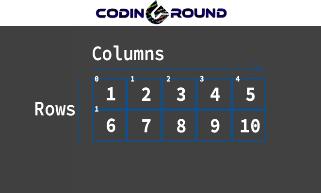
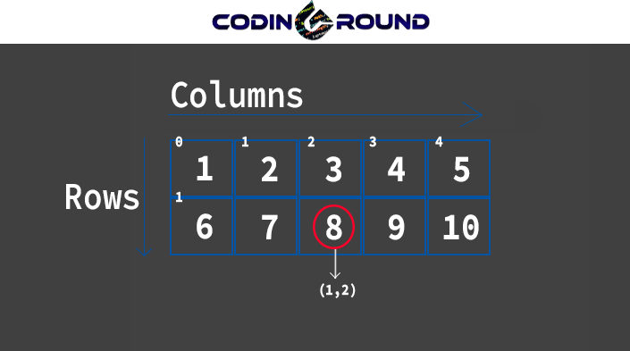
2D Arrays
a = np.array([[1,2,3,4,5],[6,7,8,9,10]])
We have created a two dimension array. Look at the image below for better understanding of how it works
Indexing in 2D array is slightly different than 1D Array. It is written like
So you first have to select the row of the element and then you select its column.
Suppose if you want to select 8 from the array then you first select its row which is 1 since it is in the second. Row and column which is 2 since it is third column
cg = np.arange(1,11).reshape(2,5)
print(cg[1,2])
Now if you want to print all the elements of the first row then you can do this by
a = np.arange(1,11).reshape(2,5)
print(a[0,:]
The Output will be
[1 2 3 4 5]
This is because you selected 1st row which is at index 0 and empty:empty which represents that you select from 0 to end with stride 1. These are default values.
These are the basics of slicing and indexing. There’s a lot to slicing but it’s all practice. You will only understand slicing when you experiment with it.
Joining Arrays
You can also join two or more arrays into a single new array. Let us consider two arrays
a1 = np.array([1,2,3])
a2 = np.array([4,5,6])
In NumPy there’s a function named concatenate() which allows us to join the arrays both horizontally and vertically. Though it must satisfy the condition.
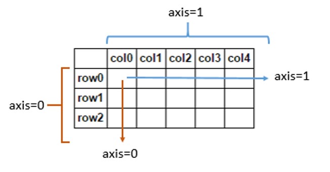
It takes 3 parameters
np.concatenate((sequence),axis,out)
Sequence: The list or tuple of arrays that you want to concatenate.
Axis(Optional): How do you want to join? Along rows or columns? By default, the axis is 0 which is rows. To join along with columns, you can change it to axis=1.
Out(Optional): If provided, the destination to place the result. The shape must be correct, matching that of what concatenate would have returned if no out argument were specified.
print(np.concatenate((a1,a2),axis=0))
The Output will be
[1 2 3 4 5 6]
Below is an image which can help you visualize axis
source: stackoverflow
Since it is a 1D Array, you can only join it in one way. If we create a 2D Array, then you will be able to join it along with both rows and columns provided it has the same number of rows or columns.
Joining along axis=0 or vstack()
For example, you cannot join an array which has 1 row with an array which has 2 rows.
You can also achieve this by using the vstack() function.
np.vstack((a1,a2))
Joining along axis=1 or hstack()
Further, if you want to join them along with columns then you can change the axis to 1. Since both arrays have the same number of rows, then you can join them along columns
You can also achieve this using the hstack() function.
np.hstack((a1,a2))
In the example, we took only 2 arrays and concatenated them but you can join as many arrays as you want. If you are starting out as a beginner, it will be more than enough for you for now. I’ll be making in-depth tutorials on each of these topics soon.
Splitting Arrays
You can also split an array into two or more arrays and store them differently. There are several functions for splitting arrays too.
The most common of them is the split () function.
split(array, indices_or_sections, axis=0)
Array: The array you want to split
Indices or Sections: Index numbers from which you want to split the array or the number of sections you want your array to split. I would recommend using sections unless it is necessary to use indices.
Axis: By which axis you’d want to split(by default it is 0).
In the case of a 1D array, you don’t really have a choice as to how you want to split it. You can only choose from which element you want to split. Let us consider a 1D array
a = np.arange(4)
Now we have an array of 4 elements. If we want to split it into two then
print(np.split(a,2))
The Output will be
[array([0, 1]), array([2, 3])]
But this function isn’t really much helpful when you are not sure about how much elements you have in array. Because it splits the elements evenly into new arrays.
For example, if you try to split this array into 3 parts then it will throw an error. To prevent that, we have another function named array_split(). Just replace split() with array_split() and it will work fine.
b = np.array_split(a,3)
print(b)
The Output will be
[array([0, 1]), array([2]), array([3])]
You can also store each array into a new variable for example
c = b[0]
d = b[1]
e = b[2]
print(c)
print(d)
print(e)
The Output will be
[0 1]
[2]
[3]
Split() is only used because it is a little faster in comparison to array_split()but it doesn’t make much of a difference in time. I would recommend using array_split() as it reduces the chances of errors.
Splitting along axis=0 or vsplit()
Let us consider a two dimensional array. We will be splitting this array along axis 0 i.e., splitting along rows.
 a1 = np.arange(1,13).reshape(2,6)
b = np.array_split(a1,2)
You can also achieve this using the hsplit() function.
np.hsplit(a1,2)
In the above example, we only split a 2D array but you can also split arrays of higher dimensions. Since it will increase the complexity to an intermediate level, we are not going to include that in this tutorial.
Comparison: Arrays, Lists and Tuples
1. Vectorized Operations: One of the main differences between Arrays, Lists, and Tuples is vectorized operations. Only Arrays allow vectorized operations i.e. when you apply a function it gets applied to each element of an array and not to array itself.
If you try the same with list or tuple it will throw a traceback error, for example:
>>>cgt = (1,2,3,4)
>>>cgt += 1
Traceback (most recent call last):
  File "<pyshell#11>", line 1, in <module>
    cgt += 1
TypeError: can only concatenate tuple (not "int") to tuple
2. Data Type Declaration: Arrays need to be declared while list, tuples, and dictionaries, etc. do not need to be declared i.e., if you want to use arrays then you have to declare them using the .array() class while you do not have to do it with lists or tuples.
3. Mutability: Mutability means the ability to be changed. Data inside arrays can be changed while the data in a tuple cannot be changed or modified.
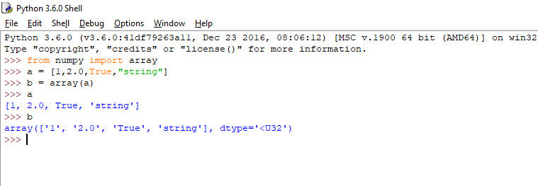
4. Heterogeneous Data: While arrays, lists, and tuples all are used to store data, arrays cannot store heterogeneous data.
If you observe carefully, the list I passed in array has each element of different data type but when printed as an array, it converted all the data as “string”. This is not the case with lists or tuples.
Array
List
Tuple
Vectorized Operations
Yes
No
No
Mutability
Yes
Yes
No
Pre-Defined Data Type
No
Yes
Yes
Heterogeneous Data
No
Yes
Yes
Features of Arrays, Lists and Tuples
When and when not to use Arrays?
When to use Arrays:
You have to store a large amount of data.
The data you want to store is of the same type.
You may perform operations on each element.
When not to use Arrays:
The Data Type is different
The data is very small
You do not have to perform operations on each element.
Highlights
First of all, congratulations on making it to the end. Now, this tutorial doesn’t really need a recap as it was kind of an overview so that you can get the hang of it. So I’ll just go through the most important of these functions which are a necessity for using NumPy.
For creating arrays, the most important functions are arange() function and the standard array() function. You may also need zeros() or ones(). I highly doubt that you will be needing any other function.
.shape is the single most important attribute of the array that you should know about. And, for adjusting shapes the .reshape() function may come in handy. It is easier to use than changing arrays shape using shape attribute.
With concatenate() function you will need to specify the axis whereas with hstack() and vstack() you do not need to type the axis. You can use either but using hstack() or vstack() may help in in future to remember the axis.
array_split() adjusts the array split according to the parameters whereas split() will throw an error if the parameters are not proper. So use array_split(). In most cases it’s a win-win. With array_split() function you will need to specify the axis whereas with hsplit() and vsplit() you do not need to specify the axis.
I guess I have covered everything important. Know that there are some sections where you might get confused if you are a first-timer. Please don’t hesitate to ask in the comments section. I will try to answer each and every comment. So, that’s all.
Speech Recognition is a hit in the market. It’s a flashy technology that is used mainly in voice assistants like Apple’s Siri, Amazon’s Alexa, Microsoft’s Cortana, Google’s Allo, etc. It can massively increase the user interaction in your project and will make it look amazing. Writing a program that uses speech recognition is far easier than you think. We will be covering everything from installing to implementation of speech recognition. Though this program will also work with Python 2, we recommend using python 3.
There’s a lot that you can do with this package but I’ll try to keep it short and cover only the most important things needed to make a simple program or to implement vocal recognition in your own program. NOTE: If you are looking just for the code then the final code is in the Conclusion section. You can view the code for Working with microphoneand Working with Audio Files directly. But if you want to know about the working of the code then you should read the article.
Introduction to Speech Recognition
Exactly What is speech recognition? In simple words, it is a technology that takes voice as an input and converts it into computer understandable language.
Setting Up
There are many modules that can be used for speech recognition like google cloud speech, apiai, SpeechRecognition, watson-developer-cloud, etc., but we will be using Speech Recognition Module for this tutorial because it is easy to use since you don’t have to code scripts for accessing audio devices also, it comes pre-packaged with many well-known API’s so you don’t have to signup for any kind of service which you may have to while using any other module. And, it gets the job done pretty well.
FLAC encoder (required only if the system is not x86-based Windows/Linux/OS X)
We will be using SpeechRecognition and PyAudio Module. *PyAudio: This module is only required if you want to take the user’s voice as an input and not use pre-recorded audio files. *PocketSphinx: Only use PocketSphinx if you have to use your program offline. I don’t personally recommend using PocketSphinx because of low accuracy.
The Speech Recognition Module
The Speech Recognition engine has support for various APIs. The most common API is Google Speech Recognition because of its high accuracy. In this tutorial though, we will be making a program using both Google Speech Recognition and CMU Sphinx so that you will have a basic idea as to how offline version works as well. However, if you want to use any other API, its pretty easy to switch, you just have to change the recognizer method(we will discuss it later in this tutorial)
Installation
I’m assuming you have python 3 properly installed. Open command prompt and type
NOTE: PyAudio is not available for python versions greater than 3.6. If you are using python 3.7 or greater then download PyAudio wheel from here.
After downloading you can install wheel file as:
pip install C:/some-dir/some-file.whl
here some-dir and some-file.whl is the directory and the file name of that wheel respectively. After installing, its always better to check the installation, open python terminal, and type
>>import speech_recognition as sr
>>sr.__version__
'3.6.0'
If it returns ‘3.6.0’ or higher then you are good to go (3.6.0 is the version that I was using because some of the libraries were not compatible with 3.7+ that I needed in my other project)
Working with Speech Recognition
After installing all the packages we are finally ready to start writing our first voice-based program. We will first be discussing the working of the speech recognition package and then we will start coding the program. You can skip to the code directly but I recommend reading the working as well because that will give you the idea about the options available that you can experiment with.
How Does it Work?
Speech Recognition has an instance named recognizer and as the name suggests it recognizes the speech(whether from an audio file or microphone). You can create a recognizer instance as follows:
import speech_recognition as sr
r = sr.Recognizer()
Note that we imported the Speech Recognition package as speech_recognition whereas we installed it as SpeechRecognition. This is a common mistake that many users make while importing this package.
Now Each Recognizer instance has eight methods by which it can recognize speech those are:
Out of these if you want to make a trigger word for your program so that it only starts and stops listening speech at a particular word(like Hey Siri or Ok Google) then you can go for Snowboy Hotword Detection. Now with speech recognition, you can do two things:
Take voice as an input from the user or
Use a pre-recorded audio file
Now for most of the people option two would be pretty useless but we will be discussing both of them in this tutorial. You can skip to the desired part of the article from the sidebar.
Using Microphone
The most awaited and most fun section finally. Writing the above part was kind of boring but it was a complete guide afterall so i had to do it.
Now for working with microphones, you need PyAudio as I mentioned above. After installing everything, you just need to type in this code.
import speech_recognition as sr
r = sr.Recognizer()

with sr.Microphone() as source:
	print("start")
	audio = r.listen(source)

	try:
		data = r.recognize_google(audio)
		print(data)
	except:
		print("Please try again")
Note: If you are using microphones other than the default one then please refer to configuring microphone settings at the bottom.
Now what we did here is we made the microphone as a source using the Microphone() method. I print start so that I would know when to start speaking. Though a symbol of mic appears in the taskbar when the program is using microphones, I did it just out of convenience.
Then we declared new variable audio that records the input. Till now the audio is only recorded through the microphone and not converted into text.
Now here comes the recognize_google() method. The recognize google method sends the audio data to the google web speech server and retrieves response.
Please note that recognize_google() uses google web speech api which is free but it is provided for testing purposes only. So I advice you not to use it for real world project.
Now there might be a time when the audio recorded just couldn’t be converted to text because of noise or other problems. If that happens then you will encounter a traceback error like this.
To prevent this from happening we put a try and except block. This checks if there is some data in the audio variable that can be converted into text. If there is some data then it completes the try block and skips the except block. If there is no data or there is some problem in parsing the data then it runs the except block.
Also, you can raise multiple exception blocks for different errors but the detailed working of try and except blocks is beyond the scope of this tutorial, so we are going to skip it.
If everything is clear to this point then changing methods is simple like if you want to use CMU Sphinx instead of google then all you have to do is replace the recognize_google() with the recognize_sphinx() method. The code would be
import speech_recognition as sr
r = sr.Recognizer()

with sr.Microphone() as source:
	print("start")
	audio = r.listen(source)

	try:
		data = r.recognize_sphinx(audio)
		print(data)
	except:
		print("Please try again")
The main reason why I recommend google web speech instead of CMU sphinx is because of the accuracy
For the same sentence “test speech recognition” both outcomes are different and it is clear the google does it better.
Using Audio Files
Working with audio files is quite similar to working with microphones. The only difference is that instead of taking voice input from the users all you have to do is pass an audio file as a source.
We will be using the sample audio that you can download from here
After downloading, place the audio file in the same folder as your program file. After that, all you have to do is instead of sr.Microphone() use sr.AudioFile(‘filename.extension’) and change the r.listen() method to r.record() method. That’s it, that’s all there is to it. You can check out the code below
import speech_recognition as sr
r = sr.Recognizer()

with sr.AudioFile('english.wav') as source:
	audio = r.record(source)
	try:
		data = r.recognize_google(audio)
		print(data)
	except:
		print("Please try again")
Conclusion
Congratulations on making it this far! This has been a long journey( at least for me haha :D) Below is the quick recap of what we did so far( cause who’s got the time to read the freakin thing again and again)
The Speech Recognition has an instance named recognizer and as the name suggests it recognizes the speech(whether from an audio file or microphone). Depending on what method you use, it process audio data accordingly. There are both online and offline methods. In online methods like recognize_google() it sends data to Google Web Speech Server whereas in recognize_sphinx() method it process data within your device.
In order to take user’s voice as an input, you need PyAudio installed. Below is the complete code for processing audio data with microphone. Note that it uses sr.Microphone() and r.listen() methods
import speech_recognition as sr
r = sr.Recognizer()
with sr.Microphone() as source:
print("start")
r.adjust_for_ambient_noise(source, duration=0.5)
audio = r.listen(source)
try:
data = r.recognize_google(audio)
print(data)
except:
print("Please try again")
Working with Audio files is similar to working with Microphones. Place the audio file that you want to process in the same directory as the program file.Below is the complete code for processing audio file. Note that it uses sr.AudioFile() and r.record() methods. Suppose you have a file name ‘english.wav’ then the code would be
import speech_recognition as sr
r = sr.Recognizer()

with sr.AudioFile('english.wav') as source:
    audio = r.record(source)
    try:
        data = r.recognize_google(audio)
        print(data)
    except:
        print("Please try again")
I tried to keep it as short and informative as possible but if I missed anything please tell me in the comments section below also if you have any doubts you can comment them down as well. I will try my best to answer you!
Miscellaneous
Configuring Microphone Settings
Note: If you are going to use your system’s default microphones then you can skip this section as there is no need to configure any microphone settings. If you want to use the microphone other than the default one then you have to select it manually.To get a list of microphones available type:
Note that the list of available microphones may vary. Now that you have a list of microphones all you have to do is select the index number of microphone. For example if you want to use Microsoft Sound Mapper which is at index number zero then all you have to do is
import speech_recognition as sr
r = sr.Recognizer()

with sr.Microphone(device_index=0) as source:
	print("start")
	audio = r.listen(source)
Reducing Noise Levels
Though you can not remove the noise completely from the background, there is adjust_for_ambient_noise() which can help you lower the noise levels in audio. For Example:
with sr.Microphone() as source: #You can also use this with audio files
	r.adjust_for_ambient_noise()
	print("start")
	audio = r.listen(source)
adjust_for_ambient_noise() reads the audio file for one second and adjusts the recognizer for the noise of that level. You can reduce the time it takes to read the audio file but it is recommended to let it read file for at least one second. But if one second seems like too much time then you can lower it by using the duration keyword. Example:
In the above example, I reduced the duration to 0.5 seconds. You can increase or decrease according to your needs. The more time you give it the better it does its work. But if you are reducing the time limit then keep it at least 0.5 seconds (the SpeechRecognition documentation recommends that)
Working with Multiple Languages
If you are using Google Web Speech then you don’t need to do anything else as it already works for almost all languages. But if you are using CMU Sphinx and need any other language pack installed then you can install addition language packs from here. All instructions for installation are mentioned on that page as well.
Writing to an Audio File
If you want to record and store user’s voice for further use(for building neural networks or maybe some other purposes) then this option is very useful for you. And this step is really easy. All you have to do is add the write command after using the r.listen() method. For example:
import speech_recognition as sr
r = sr.Recognizer()

with sr.Microphone() as source:
	print("start")
	audio = r.listen(source)

with open("microphone-results.wav","wb") as f:
	f.write(audio.get_wav_data())
This will create a file named microphone-results.wav in the same directory as the program file. With some string formatting, you can save different audio files with different names but we will cover string formatting in some other articles.
So this sums it up. Thank you for reading it till here. This article took a lot of time and energy so if you like it please tell me in the comments below. I’ll be posting more awesome articles so in order to get notified sign up for our newsletter below.